knn_euclid: Euclidean Nearest Neighbours¶

Description¶

If Y is NULL, then the function determines the first k nearest neighbours of each point in X with respect to the Euclidean distance. It is assumed that each query point is not its own neighbour.

Otherwise, for each point in Y, this function determines the k nearest points thereto from X.

Usage¶

knn_euclid(
  X,
  k = 1L,
  Y = NULL,
  algorithm = "auto",
  max_leaf_size = 0L,
  squared = FALSE,
  verbose = FALSE
)

Arguments¶


`X`	the “database”; a matrix of shape \(n\times d\)
`k`	requested number of nearest neighbours (should be rather small)
`Y`	the “query points”; `NULL` or a matrix of shape \(m\times d\); note that setting `Y=X`, contrary to `NULL`, will include the query points themselves amongst their own neighbours
`algorithm`	`"auto"`, `"kd_tree"` or `"brute"`; K-d trees can be used for `d` between 2 and 20 only; `"auto"` selects `"kd_tree"` in low-dimensional spaces
`max_leaf_size`	maximal number of points in the K-d tree leaves; smaller leaves use more memory, yet are not necessarily faster; use `0` to select the default value, currently set to 32
`squared`	whether the output `nn.dist` should be based on the squared Euclidean distance
`verbose`	whether to print diagnostic messages

Details¶

The implemented algorithms, see the algorithm parameter, assume that \(k\) is rather small, say, \(k \leq 20\).

Our implementation of K-d trees (Bentley, 1975) has been quite optimised; amongst others, it has good locality of reference (at the cost of making a copy of the input dataset), features the sliding midpoint (midrange) rule suggested by Maneewongvatana and Mound (1999), node pruning strategies inspired by some ideas from (Sample et al., 2001), and a couple of further tuneups proposed by the current author. Still, it is well-known that K-d trees perform well only in spaces of low intrinsic dimensionality. Thus, due to the so-called curse of dimensionality, for high d, the brute-force algorithm is recommended.

The number of threads used is controlled via the OMP_NUM_THREADS environment variable or via the omp_set_num_threads function at runtime. For best speed, consider building the package from sources using, e.g., -O3 -march=native compiler flags.

Value¶

A list with two elements, nn.index and nn.dist, is returned.

nn.dist and nn.index have shape \(n\times k\) or \(m\times k\), depending whether Y is given.

nn.index[i,j] is the index (between \(1\) and \(n\)) of the \(j\)-th nearest neighbour of \(i\).

nn.dist[i,j] gives the weight of the edge {i, nn.index[i,j]}, i.e., the distance between the \(i\)-th point and its \(j\)-th nearest neighbour, \(j=1,\dots,k\). nn.dist[i,] is sorted nondecreasingly for all \(i\).

Author(s)¶

Marek Gagolewski

References¶

J.L. Bentley, Multidimensional binary search trees used for associative searching, Communications of the ACM 18(9), 509–517, 1975, doi:10.1145/361002.361007.

S. Maneewongvatana, D.M. Mount, It’s okay to be skinny, if your friends are fat, 4th CGC Workshop on Computational Geometry, 1999.

N. Sample, M. Haines, M. Arnold, T. Purcell, Optimizing search strategies in K-d Trees, 5th WSES/IEEE Conf. on Circuits, Systems, Communications & Computers (CSCC’01), 2001.

Examples¶

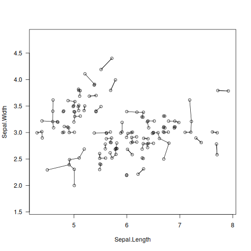
library("datasets")
data("iris")
X <- jitter(as.matrix(iris[1:2]))  # some data
neighbours <- knn_euclid(X, 1)  # 1-NNs of each point
plot(X, asp=1, las=1)
segments(X[,1], X[,2], X[neighbours$nn.index,1], X[neighbours$nn.index,2])

plot of chunk knn_euclid

knn_euclid(X, 5, matrix(c(6, 4), nrow=1))  # five closest points to (6, 4)
## $nn.index
##      [,1] [,2] [,3] [,4] [,5]
## [1,]   15   19   16   34   86
## 
## $nn.dist
##           [,1]      [,2]      [,3]      [,4]      [,5]
## [1,] 0.2159604 0.3682194 0.4916704 0.5240702 0.6041195