mst_euclid: Euclidean and Mutual Reachability Minimum Spanning Trees
Description
The function determines the/a(*) minimum spanning tree (MST) of a set of \(n\) points, i.e., an acyclic undirected connected graph whose vertices represent the points, and edges are weighted by the distances between point pairs and have minimal total weight.
MSTs have many uses in, amongst others, topological data analysis (clustering, density estimation, dimensionality reduction, outlier detection, etc.).
In clustering and density estimation, the parameter M plays the role of a smoothing factor; for discussion, see (Campello et al., 2015) and the references therein.
For \(M\leq 1\), we get a spanning tree that minimises the sum of Euclidean distances between the points, i.e., the classic Euclidean minimum spanning tree (EMST). If \(M=1\), the function additionally returns the distance to each point’s nearest neighbour.
If \(M>1\), the spanning tree is the smallest with respect to the degree-\(M\) mutual reachability distance (Campello et al., 2013) given by \(d_M(i, j)=\max\{ c_M(i), c_M(j), d(i, j)\}\), where \(d(i,j)\) is the standard Euclidean distance between the \(i\)-th and the \(j\)-th point, and \(c_M(i)\) is the \(i\)-th \(M\)-core distance defined as the distance between the \(i\)-th point and its \(M\)-th nearest neighbour (not including the query point itself).
Note that (Campello et al., 2013) defines the core distance as the distance to the \((M-1)\)-th nearest neighbour (or the \(M\)-th one, but including self).
Usage
mst_euclid(
  X,
  M = 0L,
  algorithm = "auto",
  max_leaf_size = 0L,
  first_pass_max_brute_size = 0L,
  mutreach_ties = "dist_min",
  mutreach_leaves = "keep",
  verbose = FALSE
)
Arguments
|
the “database”; a matrix of shape \(n\times d\) |
|
the smoothing factor a.k.a. the degree of the mutual reachability distance; \(M\leq 1\) gives the ordinary Euclidean distance |
|
|
|
maximal number of points in the K-d tree leaves; smaller leaves use more memory, yet are not necessarily faster; use |
|
minimal number of points in a node to treat it as a leaf (unless it actually is a leaf) in the first iteration of the algorithm; use |
|
adjustment for mutual reachability distance ambiguity (for \(M>1\)); one of |
|
a way to postprocess the leaves of the computed tree; one of |
|
whether to print diagnostic messages |
Details
(*) Note that if there are many pairs of equidistant points, there can be many minimum spanning trees. In particular, it is likely that there are point pairs with the same mutual reachability distances.
To make the definition unambiguous, the mutreach_ties argument indicates the preference towards connecting to farther/closer points with respect to the original metric, or having smaller/larger core distances in cases of tied distances; see (Gagolewski, 2026). Empirically, mutreach_ties="dcore_min" and mutreach_leaves="reconnect_dcore_min" leads to MSTs with more leaves and hubs.
The brute force method always resolves all ties, whilst, for efficiency, the K-d tree-based algorithms use this adjustment only for the first \(M\) nearest neighbours, so the resulting trees might be slightly different.
The implemented algorithms, see the algorithm parameter, assume that \(M\) is rather small.
Our implementation of K-d trees (Bentley, 1975) has been quite optimised; amongst others, it has good locality of reference (at the cost of making a copy of the input dataset), features the sliding midpoint (midrange) rule suggested by Maneewongvatana and Mound (1999), node pruning strategies inspired by some ideas from (Sample et al., 2001), and a couple of further tuneups proposed by the current author.
The “single-tree” version of the Borůvka algorithm is parallelised: in every iteration, it seeks each point’s nearest “alien”, i.e., the nearest point thereto from another cluster. The “dual-tree” Borůvka version of the algorithm is, in principle, based on (March et al., 2010). As far as our implementation is concerned, the dual-tree approach is often only faster in 2- and 3-dimensional spaces, for \(M\leq 1\), and in a single-threaded setting. For another (approximate) adaptation of the dual-tree algorithm to mutual reachability distances, see (McInnes and Healy, 2017).
The “sesqui-tree” variant (by the current author) is a mixture of the two approaches: it compares leaves against the full tree and can be run in parallel. It is usually faster than the single- and dual-tree methods in very low dimensional spaces and usually not much slower than the single-tree variant otherwise.
Nevertheless, it is well-known that K-d trees perform well only in spaces of low intrinsic dimensionality (the “curse”). For high \(d\), the “brute-force” algorithm is recommended. Here, we provided a parallelised (see Olson, 1995) version of the Jarník (1930) (a.k.a. Prim, 1957) algorithm, where the distances are computed on the fly (only once for \(M\leq 1\)).
The number of threads used is controlled via the OMP_NUM_THREADS environment variable or via the omp_set_num_threads function at runtime. For best speed, consider building the package from sources using, e.g., -O3 -march=native compiler flags.
Value
A list with two \((M=0)\) or four \((M>0)\) elements, mst.index and mst.dist, and additionally nn.index and nn.dist.
mst.index is a matrix with \(n-1\) rows and \(2\) columns, whose rows define the tree edges.
mst.dist is a vector of length \(n-1\) giving the weights of the corresponding edges.
The tree edges are ordered with respect to weights nondecreasingly, and then by the indexes (lexicographic ordering of the (weight, index1, index2) triples). For each i, it holds mst_ind[i,1]<mst_ind[i,2].
nn.index is an \(n\) by \(M\) matrix giving the indexes of each point’s nearest neighbours with respect to the Euclidean distance. nn.dist provides the corresponding Euclidean distances.
References
V. Jarník, O jistém problému minimálním, Práce Moravské Přírodovědecké Společnosti 6, 1930, 57–63.
C.F. Olson, Parallel algorithms for hierarchical clustering, Parallel Computing 21(8), 1995, 1313–1325.
R. Prim, Shortest connection networks and some generalizations, The Bell System Technical Journal 36(6), 1957, 1389–1401.
O. Borůvka, O jistém problému minimálním, Práce Moravské Přírodovědecké Společnosti 3, 1926, 37–58.
W.B. March, R. Parikshit, A.G. Gray, Fast Euclidean minimum spanning tree: Algorithm, analysis, and applications, Proc. 16th ACM SIGKDD Intl. Conf. Knowledge Discovery and Data Mining (KDD ‘10), 2010, 603–612.
J.L. Bentley, Multidimensional binary search trees used for associative searching, Communications of the ACM 18(9), 509–517, 1975, doi:10.1145/361002.361007
S. Maneewongvatana, D.M. Mount, It’s okay to be skinny, if your friends are fat, 4th CGC Workshop on Computational Geometry, 1999
N. Sample, M. Haines, M. Arnold, T. Purcell, Optimizing search strategies in K-d Trees, 5th WSES/IEEE Conf. on Circuits, Systems, Communications & Computers (CSCC’01), 2001
R.J.G.B. Campello, D. Moulavi, J. Sander, Density-based clustering based on hierarchical density estimates, Lecture Notes in Computer Science 7819, 2013, 160–172. doi:10.1007/978-3-642-37456-2_14
R.J.G.B. Campello, D. Moulavi, A. Zimek, J. Sander, Hierarchical density estimates for data clustering, visualization, and outlier detection, ACM Transactions on Knowledge Discovery from Data (TKDD) 10(1), 2015, 1–51, doi:10.1145/2733381
L. McInnes, J. Healy, Accelerated hierarchical density-based clustering, IEEE Intl. Conf. Data Mining Workshops (ICMDW), 2017, 33–42, doi:10.1109/ICDMW.2017.12
M. Gagolewski, quitefastmst, in preparation, 2026, TODO
See Also
The official online manual of quitefastmst at https://quitefastmst.gagolewski.com/
Examples
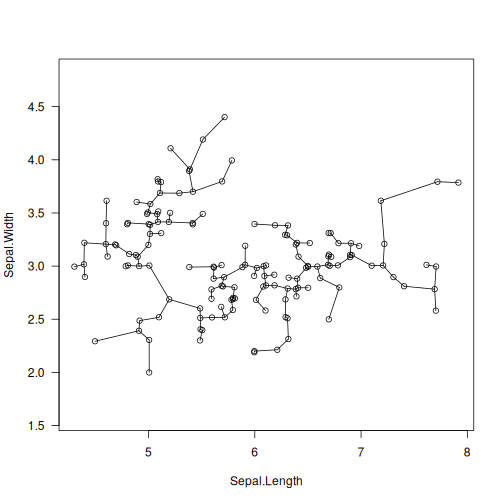
library("datasets")
data("iris")
X <- jitter(as.matrix(iris[1:2]))  # some data
T <- mst_euclid(X)                 # Euclidean MST of X
plot(X, asp=1, las=1)
segments(X[T$mst.index[, 1], 1], X[T$mst.index[, 1], 2],
         X[T$mst.index[, 2], 1], X[T$mst.index[, 2], 2])